Session 9 Review Questions
(9.1) What is the purpose of bootstrapping?
A. To calculate the exact population mean from a sample.
B. To generate multiple samples from the population without replacement.
C. To estimate the sampling distribution of the sample mean by resampling the original sample.
D. To directly calculate the confidence interval without using the sample data.
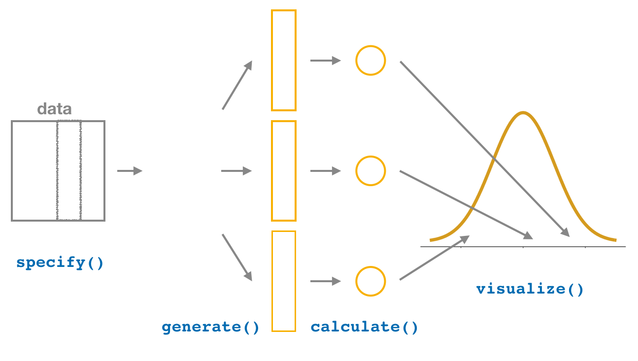
(9.2) In the bootstrapping process, what does the generate(reps = 1000, type = "bootstrap") function do?
A. It creates 1000 random samples from the original population.
B. It creates 1000 random samples with replacement from the original sample.
C. It creates 1000 exact copies of the population.
D. It creates 1000 different statistics from the original population.
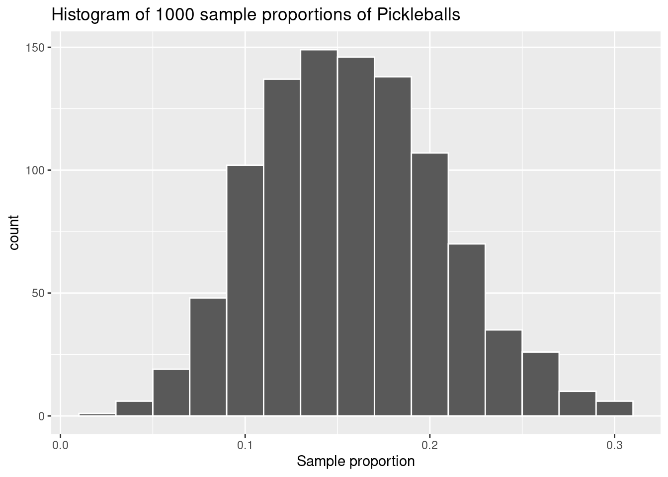
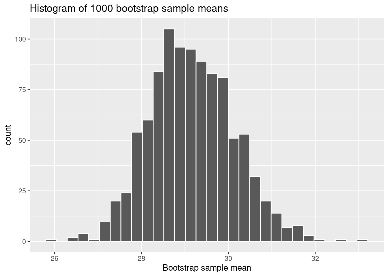
(9.3) What does the histogram of bootstrap sample means represent?
A. The distribution of sample means from the 1000 bootstrap samples.
B. The distribution of values in the original population.
C. The distribution of the population means calculated from the original sample.
D. The actual population mean with 95% certainty.
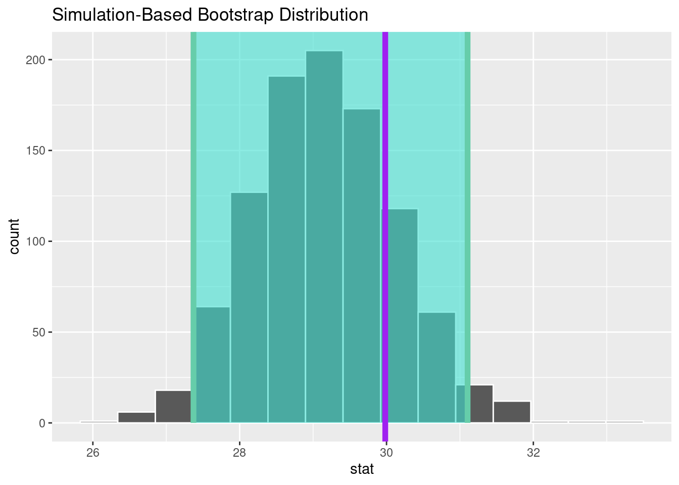
(9.4) How is the bootstrap percentile confidence interval calculated?
A. By calculating the standard deviation of the bootstrap samples.
B. By using the \(t\)-distribution to calculate the margin of error.
C. By taking the 2.5th and 97.5th percentiles of the bootstrap sample means.
D. By calculating the \(z\)-distribution based on the sample size.
(9.5) What does it mean to be “95% confident” in the bootstrap confidence interval?
A. That 95% of the bootstrap samples contain the population mean.
B. That the true population mean lies within the interval for 95% of all bootstrap samples.
C. That 95% of the population values fall within the confidence interval. D. That if we repeated the bootstrapping process many times, 95% of the confidence intervals would contain the true population mean.
Session 9 Review Question Answers
(9.1) What is the purpose of bootstrapping in the context of this commute time example?
Correct Answer:
C. To estimate the sampling distribution of the sample mean by resampling the original sample.
Explanation:
Bootstrapping allows us to approximate the sampling distribution by repeatedly resampling the original sample with replacement and calculating the statistic of interest (in this case, the mean).
(9.2) In the bootstrapping process, what does the generate(reps = 1000, type = "bootstrap") function do?
Correct Answer:
A. It generates 1000 random samples with replacement from the original sample.
Explanation:
The generate() function resamples the original data with replacement to create 1000 new bootstrap samples, which are used to estimate the sampling distribution of the sample mean.
(9.3) What does the histogram of bootstrap sample means represent?
Correct Answer:
B. The distribution of sample means from the 1000 bootstrap samples.
Explanation:
The histogram shows the variability in sample means across the 1000 bootstrap samples, giving insight into the sampling distribution of the sample mean.
(9.4) How is the bootstrap percentile confidence interval calculated?
Correct Answer:
C. By taking the 2.5th and 97.5th percentiles of the bootstrap sample means.
Explanation:
The bootstrap percentile confidence interval is found by identifying the lower and upper bounds at the 2.5th and 97.5th percentiles of the bootstrap sample means.
(9.5) What does it mean to be “95% confident” in the bootstrap confidence interval?
Correct Answer:
D. That if we repeated the bootstrapping process many times, 95% of the confidence intervals would contain the true population mean.
Explanation:
Being “95% confident” means that if we repeatedly generated bootstrap samples and calculated confidence intervals, 95% of those intervals would capture the true population mean.