Statistics in R with the tidyverse

Day 3 Exercises

Author

Dr. Chester Ismay

Day 3: Sampling and Estimation in R

Session 1: Sampling

1. Load Necessary Packages

# Load the required packages
library(dplyr)

Attaching package: 'dplyr'
The following objects are masked from 'package:stats':

    filter, lag
The following objects are masked from 'package:base':

    intersect, setdiff, setequal, union
library(ggplot2)
library(moderndive)
library(infer)
  • These packages provide tools for data wrangling, visualization, and modeling.

2. Prepare Population Dataset with Generation

# For reproducibility
set.seed(2024)

# Create vectors of sport ball types and their proportions
types_of_sport_balls <- c("Basketball", "Pickleball", "Tennis Ball", 
                          "Football/Soccer", "American Football")
proportion_of_each_type <- c(0.2, 0.15, 0.3, 0.25, 0.1)

# Create a tibble of 1200 sport balls that will act as our population
store_ball_inventory <- tibble(
  ball_ID = 1:1200,
  ball_type = sample(x = types_of_sport_balls,
                     size = 1200, 
                     replace = TRUE, 
                     prob = proportion_of_each_type
  )
)
  • We’ll be exploring a synthesized data set of an inventory at a large sporting goods store. The inventory pertains to different types of sports balls, 1200 in total.

3. Exploring Dataset Structure

# Use glimpse to explore the structure of the dataset
glimpse(store_ball_inventory)
Rows: 1,200
Columns: 2
$ ball_ID   <int> 1, 2, 3, 4, 5, 6, 7, 8, 9, 10, 11, 12, 13, 14, 15, 16, 17, 18, 19, 20, 21, 22, 23, 24, 25, 26, 27, 2…
$ ball_type <chr> "Pickleball", "Football/Soccer", "Basketball", "Basketball", "Football/Soccer", "Basketball", "Footb…

4. Population Parameters

# Create a count of ball_type
store_ball_inventory |> 
  count(ball_type)
# A tibble: 5 × 2
  ball_type             n
  <chr>             <int>
1 American Football   117
2 Basketball          252
3 Football/Soccer     299
4 Pickleball          187
5 Tennis Ball         345
# Determine the proportion of basketballs in the inventory
p_df <- store_ball_inventory |> 
  summarize(prop_bball = mean(ball_type == "Basketball"))

# Convert p to a numeric value
p <- p_df$prop_bball

# Or using the tidyverse
p <- p_df |> pull(prop_bball)
p
[1] 0.21

5. Take a Sample of Balls

# Retrieve a sample of 10 balls from the inventory
ball_sample <- store_ball_inventory |> 
  slice_sample(n = 10, replace = FALSE)

# Determine the proportion of basketballs in the sample
ball_sample |> 
  summarize(prop_bball = mean(ball_type == "Basketball"))
# A tibble: 1 × 1
  prop_bball
       <dbl>
1        0.4

6. Take Another Sample of Balls

# Retrieve another sample of 50 balls from the inventory
ball_sample2 <- store_ball_inventory |> 
  slice_sample(n = 10, replace = FALSE)

# Determine the proportion of pickleballs in the sample
ball_sample2 |> 
  summarize(prop_bball = mean(ball_type == "Basketball"))
# A tibble: 1 × 1
  prop_bball
       <dbl>
1        0.3

7. Take 1000 Samples of Size 10 from the Population

# Use `rep_slice_sample()` from the `infer` package
ball_samples <- store_ball_inventory |> 
  rep_slice_sample(n = 10, reps = 1000, replace = FALSE)
ball_samples
# A tibble: 10,000 × 3
# Groups:   replicate [1,000]
   replicate ball_ID ball_type        
       <int>   <int> <chr>            
 1         1     940 Basketball       
 2         1    1052 American Football
 3         1     749 Football/Soccer  
 4         1     497 Tennis Ball      
 5         1    1081 Tennis Ball      
 6         1     737 Basketball       
 7         1     979 Pickleball       
 8         1     944 Tennis Ball      
 9         1    1112 Tennis Ball      
10         1     855 Tennis Ball      
# ℹ 9,990 more rows

8. Calculate Sample Proportions and Visualize Them

# Determine sample proportions with `dplyr`
props_bball <- ball_samples |> 
  summarize(prop_bball = mean(ball_type == "Basketball"))

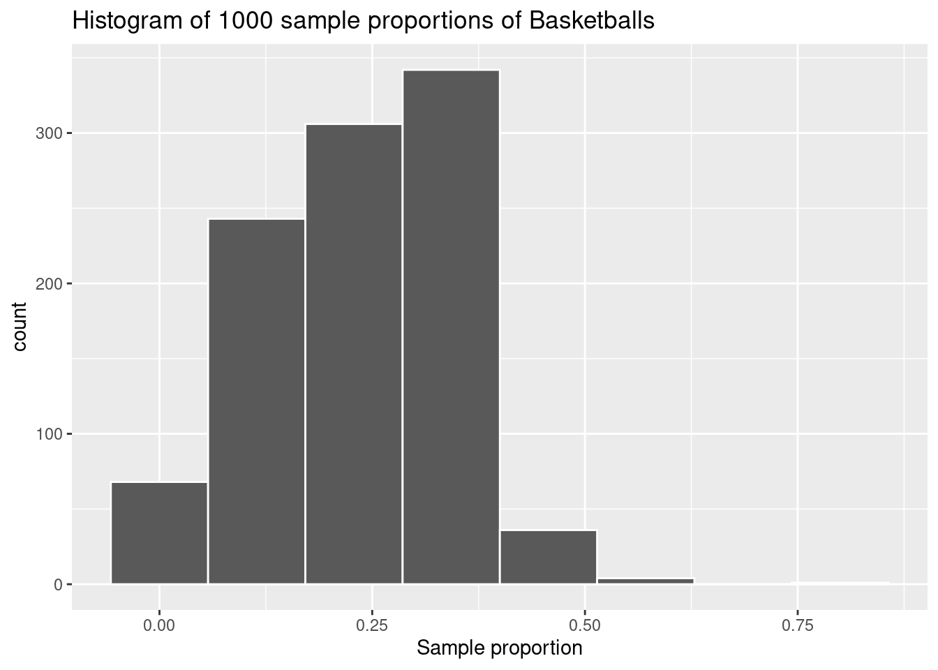
# Create a histogram of the sample proportions with 8 bins
ggplot(props_bball, aes(x = prop_bball)) +
  geom_histogram(bins = 8, color = "white") +
  labs(x = "Sample proportion", 
       title = "Histogram of 1000 sample proportions of Basketballs") 


9. Determine a Guess at the Standard Error

# Using the simulations, calculate the standard deviation of the 
# sample proportions
se_sample_props <- props_bball |> 
  summarize(sd(prop_bball)) |> 
  pull()

# Using the formula for the standard error of a sample proportion
n <- 10
se_sample_props_formula <- sqrt(p * (1 - p) / n)
se_sample_props_formula
[1] 0.1288022

10. Use Function from Walkthrough to Calculate Standard Error

# Here's the function from the walkthrough to calculate the standard error
se_sample_props <- function(size, repetitions = 1000, type = "Pickleball") {
  props <- store_ball_inventory |> 
    rep_slice_sample(n = size, reps = repetitions, replace = FALSE) |> 
    summarize(prop = mean(ball_type == type))
  
  se_sample_props <- props |> 
    summarize(sd(prop)) |> 
    pull()
  
  return(se_sample_props)
}

# Use the function to calculate the standard error for a sample size of 10
# with 2000 repetitions for Basketball
se_sample_props(10, 2000, "Basketball")
[1] 0.130401

Session 2: Estimation using Theory-based Methods

11. Population Data with Numeric Variable of Interest

Assume we have information about the population of homes in Phoenix, AZ. We are interested in their use of electricity factoring in that some homes do not have air conditioning and only use fans.

# For reproducibility
set.seed(2024)

# Number of homes in each group
n_ac <- 0.8 * 600000
n_fans <- 0.2 * 600000

# Simulate electricity usage (in kWh) for homes with AC
ac_usage <- rnorm(n_ac, mean = 1500, sd = 300)  # Higher mean for AC usage

# Simulate electricity usage (in kWh) for homes using fans
fan_usage <- rnorm(n_fans, mean = 800, sd = 150)  # Lower mean for fan usage

# Combine into a single data frame
electricity_usage_phoenix <- tibble(
  home_ID = 1:(n_ac + n_fans),
  cooling_system = c(rep("AC", n_ac), rep("Fans", n_fans)),
  usage_kWh = c(ac_usage, fan_usage)
)

# View the data
electricity_usage_phoenix
# A tibble: 600,000 × 3
   home_ID cooling_system usage_kWh
     <int> <chr>              <dbl>
 1       1 AC                 1795.
 2       2 AC                 1641.
 3       3 AC                 1468.
 4       4 AC                 1436.
 5       5 AC                 1847.
 6       6 AC                 1888.
 7       7 AC                 1660.
 8       8 AC                 1462.
 9       9 AC                 1133.
10      10 AC                 1164.
# ℹ 599,990 more rows

12. The Sample and the Sample Statistic

# Choose sample size
sample_size <- 1000

# Generate a sample
set.seed(2024)
usage_sample <- electricity_usage_phoenix |> 
  slice_sample(n = sample_size, replace = FALSE)

# Calculate the sample mean
sample_mean <- usage_sample |> 
  summarize(mean(usage_kWh)) |> 
  pull()
sample_mean
[1] 1346.212
# Calculate the standard deviation 
sample_sd <- usage_sample |> 
  summarize(sd(usage_kWh)) |> 
  pull()
sample_sd
[1] 399.186

13. Population Parameter

# Calculate the population mean
population_mean <- electricity_usage_phoenix |> 
  summarize(mean(usage_kWh)) |> 
  pull()
mu <- population_mean
mu
[1] 1360.137
# Calculate the population standard deviation
population_sd <- electricity_usage_phoenix |> 
  summarize(sd(usage_kWh)) |> 
  pull()
sigma <- population_sd
sigma
[1] 393.7991

14. Confidence Interval for the Population Proportion (Assuming We Know \(\sigma\))

# Calculate the margin of error for a 90% confidence interval
z_star <- qnorm(p = 0.95) # Assumes a normal distribution
margin_of_error <- z_star * (sigma / sqrt(sample_size))

# Recall the point estimate
point_estimate <- sample_mean

# Calculate the confidence interval
lower_bound <- point_estimate - margin_of_error
upper_bound <- point_estimate + margin_of_error

# Display the confidence interval
c(lower_bound, upper_bound)
[1] 1325.729 1366.696
# Remember the population parameter (we usually don't know it)
between(mu, lower_bound, upper_bound) # dplyr::between()
[1] TRUE

15. Confidence Interval for the Population Proportion (Assuming We Don’t Know \(\sigma\))

# Calculate the margin of error for a 90% confidence interval
t_star <- qt(p = 0.95, df = sample_size - 1) # t-distribution
margin_of_error_t <- t_star * (sample_sd / sqrt(sample_size))

# Same point estimate
point_estimate_t <- sample_mean

# Calculate the confidence interval
lower_bound_t <- point_estimate_t - margin_of_error_t
upper_bound_t <- point_estimate_t + margin_of_error_t

# Display the confidence interval
c(lower_bound_t, upper_bound_t)
[1] 1325.429 1366.995
# Remember the population parameter (we usually don't know it)
between(mu, lower_bound_t, upper_bound_t)
[1] TRUE

16. Interpreting the Confidence Interval

We are “95% confident” that the true mean commute time for this population of Phoenix houses is between 1325.4294955 and 1366.9952348 kilowatt-hours. This is the same as saying that if we were to take many samples of size 100 and calculate the confidence interval for each sample, we would expect 95% of those intervals to contain the true population mean of 1360.1370117.


Session 3: Estimation via Bootstrapping Methods

17. Assume We Only Have A Sample

# Assume we only have a sample of 1000 homes and their electricity usage
usage_sample
# A tibble: 1,000 × 3
   home_ID cooling_system usage_kWh
     <int> <chr>              <dbl>
 1   86565 AC                 1826.
 2  532090 Fans                625.
 3  127999 AC                 1738.
 4  597164 Fans                503.
 5  121242 AC                 1183.
 6   53451 AC                 1397.
 7  132457 AC                 1132.
 8  503380 Fans               1022.
 9  256276 AC                 1491.
10  418903 AC                 1201.
# ℹ 990 more rows

18. Going Over the infer Framework

Describe each step in the infer framework you have seen so far to calculate bootstrap statistics

Start with the data and then |> into the following functions:
- specify(): Define the variable of interest
- generate(): Create the bootstrap samples
- calculate(): Calculate the statistic of interest
- visualize(): Visualize the bootstrap distribution


19. Bootstrapping the Sample

# Bootstrapping the sample
set.seed(2024)
one_bootstrap <- usage_sample |> 
  specify(response = usage_kWh) |> 
  generate(reps = 1, type = "bootstrap")
one_bootstrap
Response: usage_kWh (numeric)
# A tibble: 1,000 × 2
# Groups:   replicate [1]
   replicate usage_kWh
       <int>     <dbl>
 1         1     1933.
 2         1     1733.
 3         1      947.
 4         1     1497.
 5         1     1980.
 6         1     1334.
 7         1      784.
 8         1     1175.
 9         1     1593.
10         1     1431.
# ℹ 990 more rows

20. Determine the Mean of the Bootstrap Sample

# Calculate the mean of the bootstrap sample
one_bootstrap |> 
  calculate(stat = "mean") |> 
  pull()
[1] 1332.641

21. Bootstrapping 1000 Samples

# Bootstrapping 1000 samples
many_bootstraps <- usage_sample |> 
  specify(response = usage_kWh) |> 
  generate(reps = 1000, type = "bootstrap")
many_bootstraps
Response: usage_kWh (numeric)
# A tibble: 1,000,000 × 2
# Groups:   replicate [1,000]
   replicate usage_kWh
       <int>     <dbl>
 1         1      727.
 2         1     1757.
 3         1     1343.
 4         1      796.
 5         1     1542.
 6         1     1609.
 7         1     2069.
 8         1     1044.
 9         1     2030.
10         1     1511.
# ℹ 999,990 more rows

22. Get the Mean of Each Bootstrap Sample

# Calculate the mean of each bootstrap sample
bootstrap_means <- many_bootstraps |> 
  calculate(stat = "mean")
bootstrap_means
Response: usage_kWh (numeric)
# A tibble: 1,000 × 2
   replicate  stat
       <int> <dbl>
 1         1 1357.
 2         2 1338.
 3         3 1335.
 4         4 1347.
 5         5 1340.
 6         6 1336.
 7         7 1345.
 8         8 1337.
 9         9 1372.
10        10 1377.
# ℹ 990 more rows

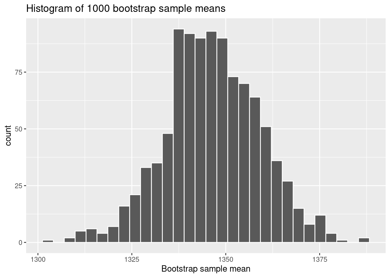
23. Visualizing the Bootstrap Distribution

# Create a histogram of the bootstrap means
ggplot(bootstrap_means, aes(x = stat)) +
  geom_histogram(bins = 30, color = "white") +
  labs(x = "Bootstrap sample mean", 
       title = "Histogram of 1000 bootstrap sample means")


24. Calculate the Bootstrap Confidence Interval

# Calculate the 90% bootstrap confidence interval in two ways since bell-shaped
bootstrap_percentile_ci <- bootstrap_means |> 
  get_confidence_interval(level = 0.90, type = "percentile")

bootstrap_se_ci <- bootstrap_means |> 
  get_confidence_interval(level = 0.90, 
                          type = "se",
                          point_estimate = sample_mean)

25. Interpretation of the Bootstrap Confidence Interval

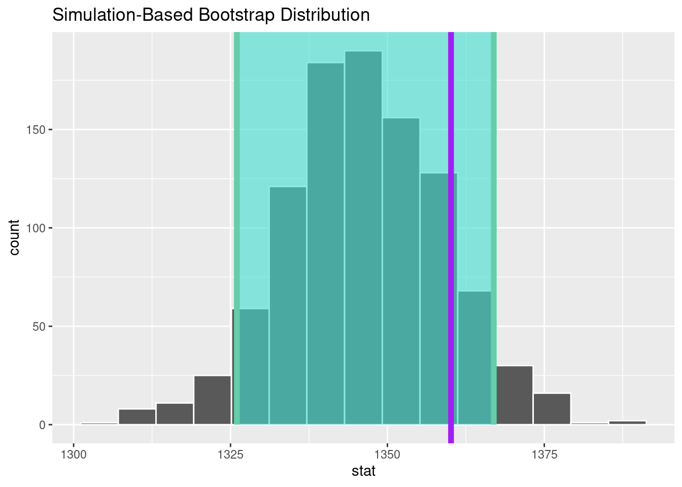
We are “95% confident” that the true mean electricity usage for this population of adults is between 1326.0090851 and 1366.9481513 kilowatt-hours. This is the same as saying that if we were to take many samples of size 100 and calculate the confidence interval for each sample, we would expect 95% of those intervals to contain the true population mean of 1360.1370117.


26. Visualize Confidence Interval on Top of Bootstrap Distribution

# Show the histogram of bootstrap means with the confidence interval
# and the population parameter (not usually known)
bootstrap_means |> 
  visualize() +
  shade_confidence_interval(endpoints = bootstrap_percentile_ci) +
  geom_vline(xintercept = mu, color = "purple", linewidth = 2)