Statistics in R with the tidyverse

Day 2 Walkthrough

Author

Dr. Chester Ismay

Day 2: Linear Regression in R

Session 4: Simple Linear Regression Analysis

1. Load Necessary Libraries

# Load the required libraries
library(dplyr)

Attaching package: 'dplyr'
The following objects are masked from 'package:stats':

    filter, lag
The following objects are masked from 'package:base':

    intersect, setdiff, setequal, union
library(ggplot2)
library(moderndive)
  • These packages provide tools for data wrangling, visualization, and modeling.

2. Prepare Dataset

library(palmerpenguins)

# Only use complete rows of data
penguins_data <- penguins |> 
  na.omit()
  • We’ll be exploring the penguins data frame from the palmerpenguins package as well. It contains size measurements for three penguin species observed on three islands in the Palmer Archipelago, Antarctica. More information is here.
  • We remove rows with missing values.

3. Exploring Dataset Structure

# Use glimpse to explore the structure of the dataset
glimpse(penguins_data)
Rows: 333
Columns: 8
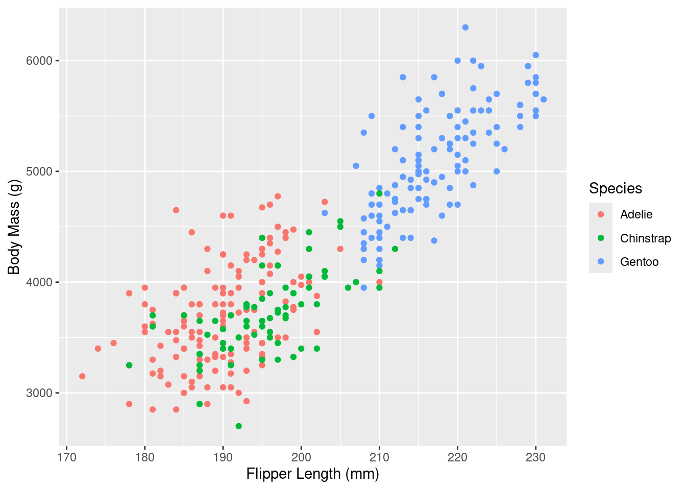
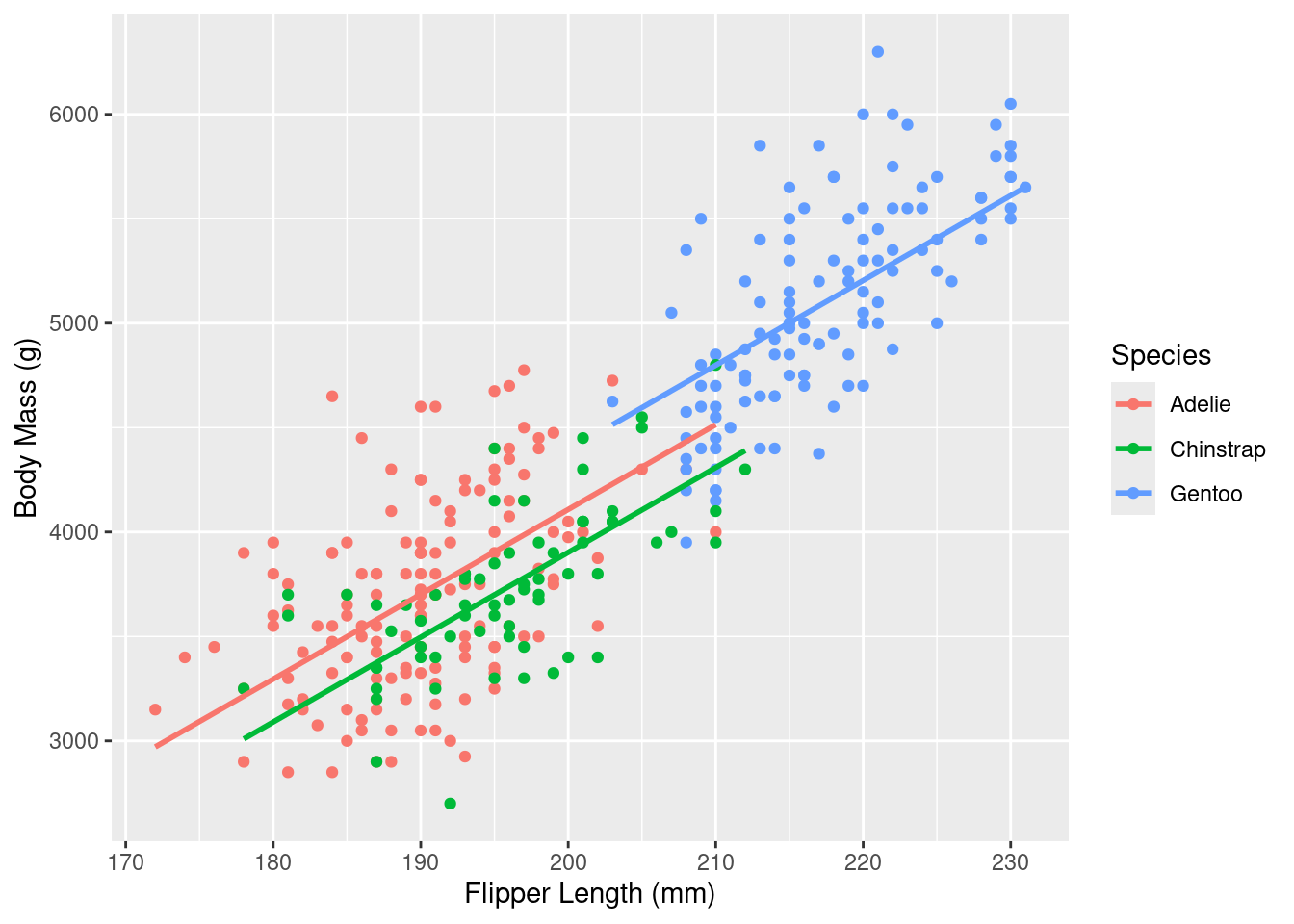
$ species           <fct> Adelie, Adelie, Adelie, Adelie, Adelie, Adelie, Adelie, Adelie, Adelie, Adelie, Adelie, Adel…
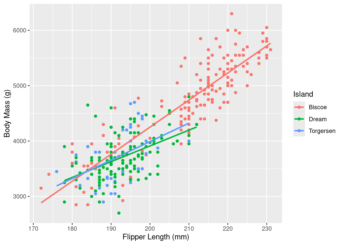
$ island            <fct> Torgersen, Torgersen, Torgersen, Torgersen, Torgersen, Torgersen, Torgersen, Torgersen, Torg…
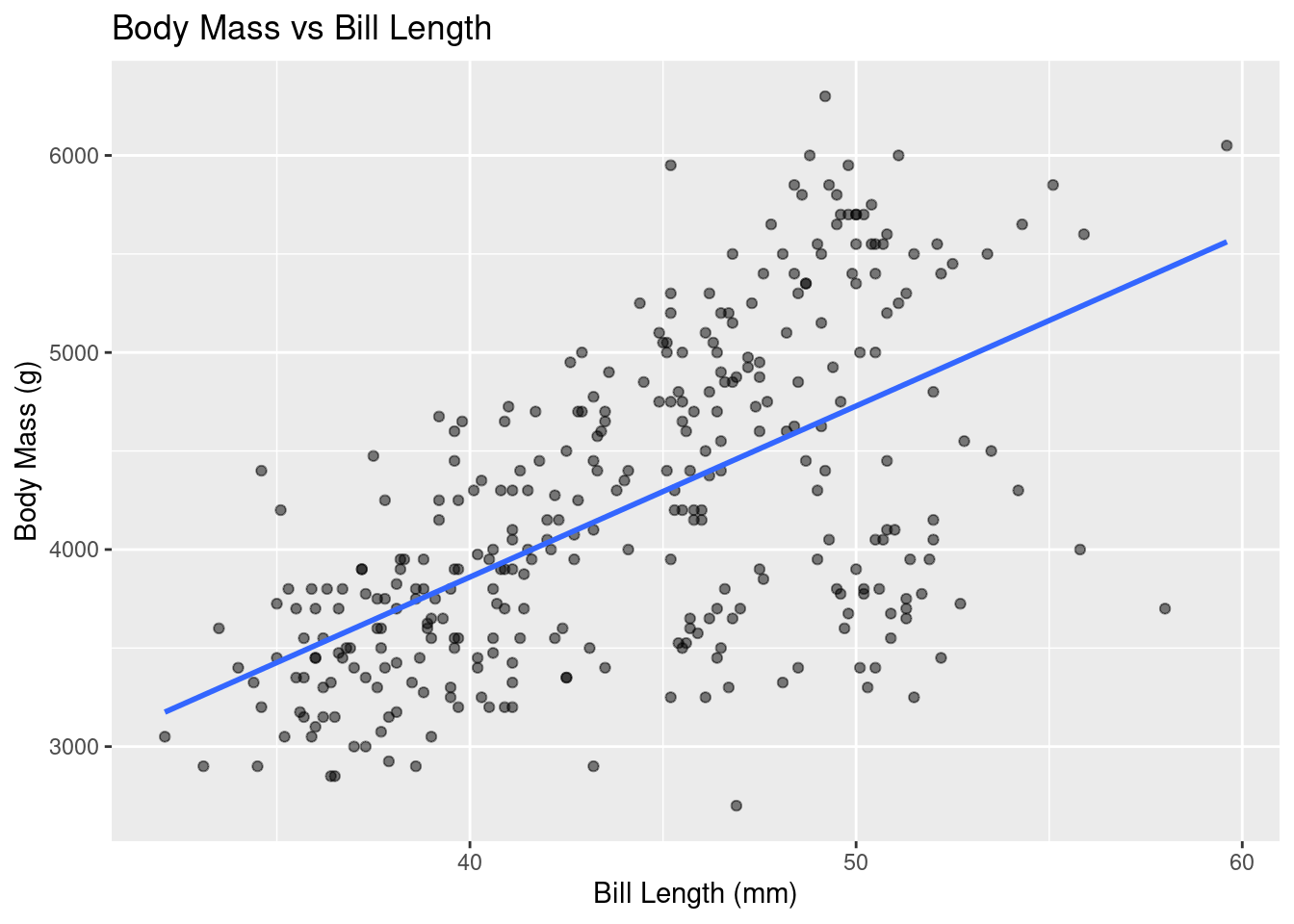
$ bill_length_mm    <dbl> 39.1, 39.5, 40.3, 36.7, 39.3, 38.9, 39.2, 41.1, 38.6, 34.6, 36.6, 38.7, 42.5, 34.4, 46.0, 37…
$ bill_depth_mm     <dbl> 18.7, 17.4, 18.0, 19.3, 20.6, 17.8, 19.6, 17.6, 21.2, 21.1, 17.8, 19.0, 20.7, 18.4, 21.5, 18…
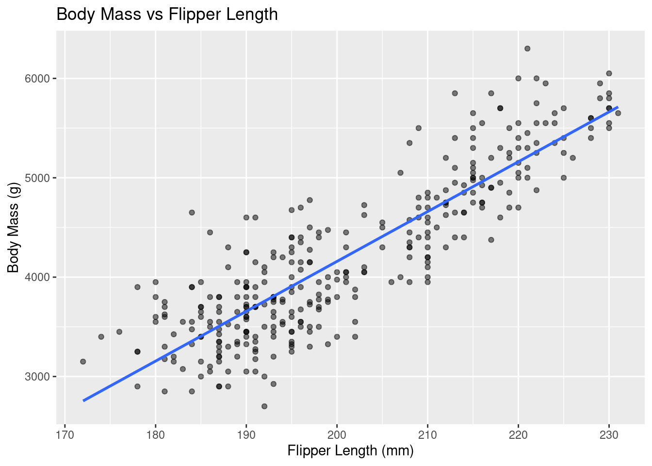
$ flipper_length_mm <int> 181, 186, 195, 193, 190, 181, 195, 182, 191, 198, 185, 195, 197, 184, 194, 174, 180, 189, 18…
$ body_mass_g       <int> 3750, 3800, 3250, 3450, 3650, 3625, 4675, 3200, 3800, 4400, 3700, 3450, 4500, 3325, 4200, 34…
$ sex               <fct> male, female, female, female, male, female, male, female, male, male, female, female, male, …
$ year              <int> 2007, 2007, 2007, 2007, 2007, 2007, 2007, 2007, 2007, 2007, 2007, 2007, 2007, 2007, 2007, 20…

The glimpse() function gives an overview of the data, showing the columns and data types.


4. Summary Statistics

# Summarize mean and median values for flipper length and body mass
penguins_data |>
  summarize(mean_flipper_length = mean(flipper_length_mm),
            mean_body_mass = mean(body_mass_g),
            median_flipper_length = median(flipper_length_mm),
            median_body_mass = median(body_mass_g))
# A tibble: 1 × 4
  mean_flipper_length mean_body_mass median_flipper_length median_body_mass
                <dbl>          <dbl>                 <int>            <int>
1                201.          4207.                   197             4050

Here, we calculate the mean and median for both flipper_length_mm and body_mass_g.


5. Using tidy_summary() Function

# Use tidy_summary to get a clean summary of the data
penguins_data |>
  select(flipper_length_mm, body_mass_g) |>
  tidy_summary()
# A tibble: 2 × 11
  column                n group type      min    Q1  mean median    Q3   max    sd
  <chr>             <int> <chr> <chr>   <int> <dbl> <dbl>  <int> <dbl> <int> <dbl>
1 flipper_length_mm   333 <NA>  numeric   172   190  201.    197   213   231  14.0
2 body_mass_g         333 <NA>  numeric  2700  3550 4207.   4050  4775  6300 805. 

The tidy_summary() function from moderndive provides a tidy summary of flipper_length_mm and body_mass_g, showing key statistics like mean, median, and standard deviation in a clean format.


6. Correlation Between Flipper Length and Body Mass

# Compute the correlation between flipper length and body mass
penguins_data |>
  get_correlation(formula = flipper_length_mm ~ body_mass_g)
# A tibble: 1 × 1
    cor
  <dbl>
1 0.873

This command calculates the correlation between flipper_length_mm and body_mass_g.


7. Scatterplot of Flipper Length and Body Mass

# Plot the relationship between flipper length and body mass
ggplot(penguins_data, aes(x = flipper_length_mm, y = body_mass_g)) +
  geom_point(alpha = 0.5) +
  labs(x = "Flipper Length (mm)", y = "Body Mass (g)",
       title = "Scatterplot of Flipper Length and Body Mass")

This scatterplot shows the relationship between flipper length and body mass.


8. Regression Line

# The same scatterplot with a regression line added
ggplot(penguins_data, aes(x = flipper_length_mm, y = body_mass_g)) +
  geom_point(alpha = 0.5) +
  geom_smooth(method = "lm", se = FALSE) +
  labs(x = "Flipper Length (mm)", y = "Body Mass (g)",
       title = "Flipper Length vs. Body Mass with Regression Line")
`geom_smooth()` using formula = 'y ~ x'

This scatterplot includes a linear regression line to show the trend in the data.


9. Fit a Regression Model

# Fit a linear regression model
flipper_model <- lm(body_mass_g ~ flipper_length_mm, data = penguins_data)

# Get the regression coefficients
coef(flipper_model)
      (Intercept) flipper_length_mm 
      -5872.09268          50.15327 

Here, we fit a linear model to predict body_mass_g using flipper_length_mm and extract the coefficients of the model.


Session 4 Review Questions

(4.1) What is the purpose of the na.omit() function in the code below?

penguins_data <- penguins |>
  select(species, island, flipper_length_mm, body_mass_g) |>
  na.omit()

A. It replaces missing values with the median.
B. It removes any rows that contain missing values.
C. It converts missing values to zeros.
D. It fills missing values with the previous non-missing value.


(4.2) What does the tidy_summary() function do when applied to numeric columns in the penguins_data data frame?

A. It generates summary statistics for each column in the data frame.
B. It prints the first 6 rows of the data frame.
C. It provides a compact overview of the data, including column names and data types.
D. It creates a scatterplot of the variables in the data frame.


(4.3) Which of the following correctly calculates the mean body mass in the penguins_data data frame?

A. summarize |> penguins_data(mean_flipper = mean(body_mass_g))
B. summarize(mean(body_mass_g))
C. summarize(penguins_data, mean = body_mass_g) D. penguins_data |> summarize(mean_body_mass = mean(body_mass_g))


(4.4) What does the get_correlation() function do when applied in the code below?

penguins_data |>
  get_correlation(formula = flipper_length_mm ~ body_mass_g)

A. It fits a linear regression model.
B. It gives a measure of the linear relationship between flipper length and body mass. C. It plots a scatterplot of flipper length and body mass.
D. It generates summary statistics for flipper length and body mass.


(4.5) In the following code, what is the purpose of geom_smooth(method = "lm", se = FALSE)?

ggplot(penguins_data, aes(x = flipper_length_mm, y = body_mass_g)) +
  geom_point(alpha = 0.5) +
  geom_smooth(method = "lm", se = FALSE) +
  labs(x = "Flipper Length (mm)", y = "Body Mass (g)",
       title = "Flipper Length vs. Body Mass with Regression Line")

A. It adds a smoothed curve based on a polynomial fit to the scatterplot.
B. It adds a linear regression line to the scatterplot without displaying the confidence interval.
C. It adjusts the transparency of the points in the scatterplot.
D. It calculates and displays residuals on the plot.


Session 4 Review Question Answers

(4.1) What is the purpose of the na.omit() function in the code below?

Correct Answer:
B. It removes any rows that contain missing values.

Explanation:
The na.omit() function is used to filter out rows that have missing values, ensuring the analysis is performed on complete cases only.


(4.2) What does the tidy_summary() function do when applied to numeric columns in the penguins_data data frame?

Correct Answer:
A. It generates summary statistics for each column in the data frame.

Explanation:
tidy_summary() in the moderndive package produces summary statistics for each selected numeric column in the data frame provided.


(4.3) Which of the following correctly calculates the mean body mass in the penguins_data data frame?

Correct Answer:
D. penguins_data |> summarize(mean_body_mass = mean(body_mass_g)

Explanation:
The correct syntax includes both column names and calculated statistics for each variable using the summarize() function.


(4.4) What does the get_correlation() function do when applied in the code below?

penguins_data |>
  get_correlation(formula = flipper_length_mm ~ body_mass_g)

Correct Answer:
B. It gives a measure of the linear relationship between flipper length and body mass.

Explanation:
The get_correlation() function computes the correlation coefficient between the two specified variables, indicating the strength and direction of their linear relationship.


(4.5) In the following code, what is the purpose of geom_smooth(method = "lm", se = FALSE)?

ggplot(penguins_data, aes(x = flipper_length_mm, y = body_mass_g)) +
  geom_point(alpha = 0.5) +
  geom_smooth(method = "lm", se = FALSE) +
  labs(x = "Flipper Length (mm)", y = "Body Mass (g)",
       title = "Flipper Length vs. Body Mass with Regression Line")

Correct Answer:
B. It adds a linear regression line to the scatterplot without displaying the confidence interval.

Explanation:
geom_smooth(method = "lm") fits a linear model to the data, and se = FALSE suppresses the shaded confidence interval around the regression line.


Session 5: Multiple Linear Regression Analysis (Part 1)

10: Fitting a Simple Linear Regression with a Categorical Regressor

# Fit a simple linear regression model with species as a predictor
species_model <- lm(body_mass_g ~ species, data = penguins_data)

# Get regression coefficients
coef(species_model)
     (Intercept) speciesChinstrap    speciesGentoo 
      3706.16438         26.92385       1386.27259 

Explanation: We fit a simple linear regression model to predict body_mass_g using species as a categorical predictor. The coefficients represent the differences in body mass between the species with a baseline set as the first species alphabetically (Adélie).


11: Visualizing Data with Categorical Variables

# Scatterplot with species as color for grouping
ggplot(penguins_data, 
       aes(x = flipper_length_mm, y = body_mass_g, color = species)) +
  geom_point() +
  labs(x = "Flipper Length (mm)", y = "Body Mass (g)", color = "Species")

Explanation:
We create a scatterplot to visualize the relationship between flipper_length_mm and body_mass_g, using species as a color grouping. This allows us to see how the relationship varies across penguin species.


12: Summarizing the Target and Regressors (One numerical and one categorical)

# Summarize the target and regressors
penguins_data |>
  select(body_mass_g, flipper_length_mm, species) |>
  tidy_summary()
# A tibble: 5 × 11
  column                n group     type      min    Q1  mean median    Q3   max    sd
  <chr>             <int> <chr>     <chr>   <dbl> <dbl> <dbl>  <dbl> <dbl> <dbl> <dbl>
1 body_mass_g         333 <NA>      numeric  2700  3550 4207.   4050  4775  6300 805. 
2 flipper_length_mm   333 <NA>      numeric   172   190  201.    197   213   231  14.0
3 species             146 Adelie    factor     NA    NA   NA      NA    NA    NA  NA  
4 species              68 Chinstrap factor     NA    NA   NA      NA    NA    NA  NA  
5 species             119 Gentoo    factor     NA    NA   NA      NA    NA    NA  NA  

Explanation:
We use tidy_summary() to summarize the target variable body_mass_g and the regressors flipper_length_mm and species. This provides a concise overview of the data, including key statistics for each variable. Note that species only lists the three levels of the group since the remaining columns correspond to numeric variables only.


13: Fitting a Multiple Regression Model with Interaction Terms

# Fit a multiple regression model with interaction
multi_model_interaction <- lm(body_mass_g ~ flipper_length_mm * species, 
                              data = penguins_data)

# Get regression coefficients
coef(multi_model_interaction)
                       (Intercept)                  flipper_length_mm                   speciesChinstrap 
                       -2508.08774                           32.68891                         -529.10803 
                     speciesGentoo flipper_length_mm:speciesChinstrap    flipper_length_mm:speciesGentoo 
                       -4166.11653                            1.88448                           21.47651 

Explanation:
We fit a multiple regression model that includes both flipper_length_mm and species as predictors of body_mass_g. The * symbol indicates that we are fitting both main effects and interaction terms. The regression coefficients reflect the impact of both the flipper length and the species on body mass as well as the interaction between flipper length and species.

In the fitted model, species is represented as dummy variables. For example, the coefficient for speciesChinstrap shows how being a Chinstrap penguin affects body mass relative to the baseline species (Adélie). Similarly, the interaction terms (e.g., flipper_length_mm:speciesGentoo) tell us how the relationship between flipper length and body mass changes for each species compared to the baseline.

In this model (multi_model_interaction), we’ve included an interaction term between flipper_length_mm and species. This interaction term allows the effect of flipper length on body mass to differ depending on the species of penguin. Here’s how to interpret the coefficients:

Model Overview:

The model is predicting body_mass_g (body mass of penguins in grams) based on flipper_length_mm (flipper length in millimeters), species, and their interaction (flipper_length_mm * species). The interaction term means that the relationship between flipper length and body mass can change depending on the species.

1. (Intercept): -2508.09

  • This is the predicted body mass for an Adelie penguin (the reference category for species) when its flipper length is 0. Again, this may not be realistic, but it provides a baseline for interpretation.

2. flipper_length_mm: 32.69

  • For Adelie penguins, each additional millimeter in flipper length increases their predicted body mass by about 32.69 grams. This coefficient represents the slope of flipper_length_mm for the reference species (Adelie).

3. speciesChinstrap: -529.11

  • This is the difference in the baseline body mass between Chinstrap penguins and Adelie penguins when flipper length is 0. Chinstrap penguins are predicted to weigh 529.11 grams less than Adelie penguins at the same flipper length of 0.

4. speciesGentoo: -4166.12

  • Similarly, Gentoo penguins are predicted to weigh 4166.12 grams less than Adelie penguins at a flipper length of 0. This is a large value, but remember that the intercept applies to the scenario where flipper length is 0, which may not be relevant in practice.

5. flipper_length_mm:speciesChinstrap: 1.88

  • This is the interaction effect. It shows how the relationship between flipper length and body mass changes for Chinstrap penguins compared to Adelie penguins.
  • For Chinstrap penguins, each additional millimeter in flipper length is associated with an additional increase of 1.88 grams in body mass on top of the 32.69 grams increase for Adelie penguins. So the total effect of flipper length on body mass for Chinstrap penguins is 32.69 + 1.88 = 34.57 grams per millimeter of flipper length.

6. flipper_length_mm:speciesGentoo: 21.48

  • This interaction term shows how the relationship between flipper length and body mass changes for Gentoo penguins compared to Adelie penguins.
  • For Gentoo penguins, each additional millimeter in flipper length is associated with an additional increase of 21.48 grams in body mass on top of the 32.69 grams increase for Adelie penguins. So the total effect of flipper length on body mass for Gentoo penguins is 32.69 + 21.48 = 54.17 grams per millimeter of flipper length.

Summary of Interpretation:

  • For Adelie penguins, each additional millimeter in flipper length increases body mass by about 32.69 grams.
  • For Chinstrap penguins, the increase in body mass per millimeter of flipper length is slightly higher, at about 34.57 grams (32.69 + 1.88).
  • For Gentoo penguins, the increase in body mass per millimeter of flipper length is even higher, at about 54.17 grams (32.69 + 21.48).
  • The baseline (intercept) body mass for Chinstrap and Gentoo penguins is lower than for Adelie penguins, but this only applies when flipper length is 0 (which is not a realistic flipper length but is the mathematical interpretation).

By including the interaction term, this model reveals that the relationship between flipper length and body mass differs across species.


14: Adding Interaction Terms to the Regression Plot

# Scatterplot with regression lines by species
ggplot(penguins_data, aes(x = flipper_length_mm, y = body_mass_g, color = species)) +
  geom_point() +
  geom_smooth(method = "lm", se = FALSE) +
  labs(x = "Flipper Length (mm)", y = "Body Mass (g)", color = "Species")
`geom_smooth()` using formula = 'y ~ x'

Explanation:
We extend the scatterplot by adding regression lines for each species, showing how the relationship between flipper_length_mm and body_mass_g differs across species. Each line represents a separate slope for each species, which reflects the interaction between flipper length and species in the model.


Session 5 Review Questions

(5.1) What is the default baseline island in the simple linear regression model for predicting body_mass_g using island as a categorical variable?

A. Torgersen
B. Biscoe
C. Dream
D. The island with the highest body mass


(5.2) In the following regression model with interaction terms, what does the coefficient for flipper_length_mm:speciesGentoo represent?

multi_model_interaction <- lm(body_mass_g ~ flipper_length_mm * species, data = penguins_data)

A. The slope of the regression line for Gentoo penguins
B. The average body mass of Gentoo penguins
C. The change in the relationship between flipper length and body mass for Gentoo penguins compared to the baseline
D. The difference in intercept for Gentoo penguins compared to the baseline


(5.3) What is the purpose of adding interaction terms to a multiple regression model?

A. To make the model more complex without any real benefit
B. To estimate the relationship between each explanatory variable and the response variable independently
C. To account for how the relationship between one explanatory variable and the response depends on another explanatory variable
D. To automatically improve the model’s R-squared value


(5.4) What does the following plot indicate about the relationship between flipper length and body mass for different islands?

ggplot(penguins_data, aes(x = flipper_length_mm, y = body_mass_g, color = island)) +
  geom_point() +
  geom_smooth(method = "lm", se = FALSE) +
  labs(x = "Flipper Length (mm)", y = "Body Mass (g)", color = "Island")
`geom_smooth()` using formula = 'y ~ x'

A. The relationship between flipper length and body mass is the same for all islands
B. The relationship between flipper length and body mass differs across species, with each island having a different slope
C. The islands do not influence the relationship between flipper length and body mass
D. Only the intercept differs for each island, but the slope is the same


(5.5) In the multiple regression model with interaction terms, how are dummy variables used for categorical predictors?

A. Dummy variables are used to represent the different categories of a categorical variable B. Dummy variables are used to represent each numerical variable
C. Dummy variables are used to replace the intercept in the regression model
D. Dummy variables are not necessary for categorical variables


Session 5 Review Question Answers

(5.1) What is the default baseline island in the simple linear regression model for predicting body_mass_g using island as a categorical variable?

Correct Answer:
B. Biscoe

Explanation:
In a regression model with categorical variables, the baseline group is typically the first level alphabetically. Since Biscoe comes first, it is the baseline for comparison.


(5.2) In the following regression model with interaction terms, what does the coefficient for flipper_length_mm:speciesGentoo represent?

Correct Answer:
D. The change in the relationship between flipper length and body mass for Gentoo penguins compared to the baseline

Explanation:
The interaction term flipper_length_mm:speciesGentoo represents how the effect of flipper_length_mm on body_mass_g changes for Gentoo penguins compared to the baseline species, Adélie.


(5.3) What is the purpose of adding interaction terms to a multiple regression model?

Correct Answer:
C. To account for how the relationship between one explanatory variable and the response depends on another explanatory variable

Explanation:
Interaction terms allow us to model how the effect of one predictor (e.g., flipper length) on the outcome (body mass) changes depending on the level of another predictor (e.g., species).


(5.4) What does the following plot indicate about the relationship between flipper length and body mass for different islands?

ggplot(penguins_data, aes(x = flipper_length_mm, y = body_mass_g, color = island)) +
  geom_point() +
  geom_smooth(method = "lm", se = FALSE) +
  labs(x = "Flipper Length (mm)", y = "Body Mass (g)", color = "Island")
`geom_smooth()` using formula = 'y ~ x'

Correct Answer:
B. The relationship between flipper length and body mass differs across species, with each species having a different slope

Explanation:
The plot shows separate regression lines for each species, indicating that the relationship between flipper_length_mm and body_mass_g varies by species, with each species having a unique slope.


(5.5) In the multiple regression model with interaction terms, how are dummy variables used for categorical predictors?

Correct Answer:
A. Dummy variables are used to represent the different categories of a categorical variable

Explanation:
In regression models, dummy variables are created for categorical variables like species to represent the different levels (e.g., Adélie, Chinstrap, Gentoo) in the model. These dummy variables allow the model to estimate how each category affects the outcome relative to the baseline category.


Session 6: Multiple Linear Regression Analysis (Part 2)

15. Fitting a Multiple Regression Model Without Interactions

# Fit a multiple regression model without interaction terms
multi_model_no_interaction <- lm(body_mass_g ~ flipper_length_mm + species, 
                              data = penguins_data)

# Get regression coefficients
coef(multi_model_no_interaction)
      (Intercept) flipper_length_mm  speciesChinstrap     speciesGentoo 
      -4013.17889          40.60617        -205.37548         284.52360 

Explanation:

  • We fit a multiple regression model predicting body_mass_g (body mass) using both flipper_length_mm (flipper length) and species as explanatory variables.
  • In this model, the effect of each explanatory variable on body mass is assumed to be independent, meaning the slopes are the same across different levels of the other variable (i.e., no interaction).
  • The coefficients indicate the effect of each predictor on body mass, with each variable having its own impact on the response.

The output from our linear regression model (multi_model_no_interaction) can be interpreted as follows:

Model Overview:

The model is predicting body_mass_g (the body mass of penguins in grams) based on flipper_length_mm (flipper length in millimeters) and species. Since the species variable is categorical, the model automatically creates dummy variables for the species, treating one species (Adelie) as the reference category.

Let’s break down each coefficient:

1. (Intercept): -4013.18

  • This is the predicted body mass (in grams) for a penguin that belongs to the reference species Adelie and has a flipper_length_mm of 0 (which may not be realistic in this context, but it’s the mathematical meaning).
  • In simpler terms, it provides a baseline body mass for the reference species when other variables (like flipper length) are zero.

2. flipper_length_mm: 40.61

  • For each additional millimeter in flipper length, the model predicts an increase of approximately 40.61 grams in body mass, holding the species constant.
  • This means that flipper length has a positive effect on body mass.

3. speciesChinstrap: -205.38

  • Chinstrap penguins are expected to have, on average, body masses that are 205.38 grams lower than Adelie penguins (the reference species), holding flipper_length_mm constant.
  • This represents the difference between the Chinstrap species and the Adelie species in terms of body mass, after accounting for flipper length.

4. speciesGentoo: 284.52

  • Gentoo penguins are expected to have, on average, body masses that are 284.52 grams higher than Adelie penguins, holding flipper_length_mm constant.
  • This shows that, after adjusting for flipper length, Gentoo penguins tend to be heavier than the Adelie species.

Summary of Interpretation:

  • The model suggests that penguin body mass increases as flipper length increases.
  • Chinstrap penguins tend to have lower body masses than Adelie penguins (reference category), while Gentoo penguins tend to have higher body masses compared to Adelie penguins, even after accounting for differences in flipper length.

16. Visualizing the Parallel Slopes Model

# Scatterplot with regression lines by species (different intercepts but same slopes)
ggplot(penguins_data, aes(x = flipper_length_mm, y = body_mass_g, color = species)) +
  geom_point() +
  geom_parallel_slopes(se = FALSE) +
  labs(x = "Flipper Length (mm)", y = "Body Mass (g)", color = "Species")

Explanation:

  • We visualize the fitted multiple regression model without interactions using parallel slope lines.
  • The function geom_parallel_slopes() is used to create regression lines with the same slope for each species.
  • This helps to visualize the idea of parallel slopes, where each regression line has the same slope but different intercepts depending on the other explanatory variable (flipper length).

17. Summarize the Numerical Regressors and Target Variable

# Use tidy_summary to get a clean summary of the data for a multiple regression
# with flipper length and bill length and regressors and body mass as the
# outcome
penguins_data |>
  select(body_mass_g, flipper_length_mm, bill_length_mm) |>
  tidy_summary()
# A tibble: 3 × 11
  column                n group type       min     Q1   mean median     Q3    max     sd
  <chr>             <int> <chr> <chr>    <dbl>  <dbl>  <dbl>  <dbl>  <dbl>  <dbl>  <dbl>
1 body_mass_g         333 <NA>  numeric 2700   3550   4207.  4050   4775   6300   805.  
2 flipper_length_mm   333 <NA>  numeric  172    190    201.   197    213    231    14.0 
3 bill_length_mm      333 <NA>  numeric   32.1   39.5   44.0   44.5   48.6   59.6   5.47

This provides a tidy summary, giving key statistics such as the mean, median, and standard deviation for the selected variables.


18. Fitting a Multiple Regression Model with Two Numerical Predictors

# Fit a multiple regression model
multi_model <- lm(body_mass_g ~ flipper_length_mm + bill_length_mm, 
                  data = penguins_data)

# Get regression coefficients
coef(multi_model)
      (Intercept) flipper_length_mm    bill_length_mm 
     -5836.298732         48.889692          4.958601 

In this multiple regression model, we predict body_mass_g using both flipper_length_mm and bill_length_mm. The coefficients show the effect of each variable on the response.


19. Visualizing the Relationship between Variables (with SLR)

# Create scatterplot with regression lines for both variables
ggplot(penguins_data, aes(x = flipper_length_mm, y = body_mass_g)) +
  geom_point(alpha = 0.5) +
  geom_smooth(method = "lm", se = FALSE) +
  labs(x = "Flipper Length (mm)", y = "Body Mass (g)",
       title = "Body Mass vs Flipper Length")
`geom_smooth()` using formula = 'y ~ x'

ggplot(penguins_data, aes(x = bill_length_mm, y = body_mass_g)) +
  geom_point(alpha = 0.5) +
  geom_smooth(method = "lm", se = FALSE) +
  labs(x = "Bill Length (mm)", y = "Body Mass (g)",
       title = "Body Mass vs Bill Length")
`geom_smooth()` using formula = 'y ~ x'

These scatterplots display the relationships individually between flipper_length_mm and body_mass_g, and between bill_length_mm and body_mass_g, with linear regression lines added.


Session 6 Review Questions

(6.1) What is the main assumption in a multiple regression model without interaction terms?

A. The relationship between the explanatory variables and the response is always quadratic.
B. The slope of the regression line is different for each level of the categorical variable.
C. The slope of the regression line is the same for all levels of the categorical variable.
D. The intercept of the regression line is the same for all levels of the categorical variable.


(6.2) In the model lm(body_mass_g ~ flipper_length_mm + species, data = penguins_data), what does the coefficient for speciesGentoo represent?

A. The effect of being a Gentoo penguin on body mass compared to the baseline species (Adélie).
B. The effect of flipper length on body mass for Gentoo penguins only.
C. The change in flipper length due to species.
D. The effect of body mass on flipper length for Gentoo penguins.


(6.3) What does the function geom_parallel_slopes() do in a regression plot?

A. It fits regression lines with different slopes for each group.
B. It plots regression lines with the same slope but different intercepts for each group.
C. It creates a scatterplot without any regression lines.
D. It visualizes interaction effects between the variables.


(6.4) In the model lm(body_mass_g ~ flipper_length_mm + bill_length_mm, data = penguins_data), what do the coefficients for flipper_length_mm and bill_length_mm represent?

A. The total body mass of each penguin species.
B. The predicted body mass for penguins with average bill and flipper lengths. C. The interaction effect between flipper length and bill length.
D. The effect of bill length on body mass, controlling for flipper length, and vice versa.


(6.5) What does a regression model without interaction terms assume about the relationship between the explanatory variables and the response variable?

A. The explanatory variables are not related to the response.
B. The relationship between the explanatory variables and the response is independent of one another.
C. The explanatory variables interact to affect the response.
D. The response variable depends only on the categorical variables.


Session 6 Review Question Answers

(6.1) What is the main assumption in a multiple regression model without interaction terms?

Correct Answer:
C. The slope of the regression line is the same for all levels of the categorical variable.

Explanation:
In a multiple regression model without interactions, the slopes are assumed to be the same across all levels of the categorical variable. Only the intercepts are allowed to differ by group.


(6.2) In the model lm(body_mass_g ~ flipper_length_mm + species, data = penguins_data), what does the coefficient for speciesGentoo represent?

Correct Answer:
A. The effect of being a Gentoo penguin on body mass compared to the baseline species (Adélie).

Explanation:
In regression models with categorical variables, the coefficient for a level like speciesGentoo represents the difference in the response variable (body mass) for Gentoo penguins compared to the baseline species (Adélie).


(6.3) What does the function geom_parallel_slopes() do in a regression plot?

Correct Answer:
B. It plots regression lines with the same slope but different intercepts for each group.

Explanation:
The geom_parallel_slopes() function is used to visualize regression models without interaction terms, where each group has the same slope but different intercepts.


(6.4) In the model lm(body_mass_g ~ flipper_length_mm + bill_length_mm, data = penguins_data), what do the coefficients for flipper_length_mm and bill_length_mm represent?

Correct Answer:
D. The effect of bill length on body mass, controlling for flipper length, and vice versa.

Explanation:
In a multiple regression model, each coefficient represents the effect of that variable on the response, while controlling for the other variables in the model.


(6.5) What does a regression model without interaction terms assume about the relationship between the explanatory variables and the response variable?

Correct Answer:
B. The relationship between the explanatory variables and the response is independent of one another.

Explanation:
In a regression model without interaction terms, it is assumed that the explanatory variables affect the response independently, meaning that the effect of one variable is not influenced by the level of the other.