Statistics in R with the tidyverse

Day 2 Exercises

Author

Dr. Chester Ismay

Day 2: Linear Regression in R

Session 4: Simple Linear Regression Analysis

1. Load Necessary Libraries

We did this during the course in walkthroughs, but if you haven’t done it yet:

# Load the required libraries
library(dplyr)

Attaching package: 'dplyr'
The following objects are masked from 'package:stats':

    filter, lag
The following objects are masked from 'package:base':

    intersect, setdiff, setequal, union
library(ggplot2)
library(moderndive)
library(readr)
  • These packages provide tools for data wrangling, visualization, and modeling.

2. Prepare Dataset

# Load in the data_dev_survey CSV file as a data frame again
# selecting the columns of interest keeping only complete rows of information
data_dev_survey <- read_csv("../data_dev_survey.csv") |> 
  select(response_id, converted_comp_yearly, work_exp, 
         years_code, ai_trust) |> 
  # This code sets the levels of the ai_trust column to be more intuitive
  # Note this will change the baseline level for the factor!
  mutate(ai_trust = factor(ai_trust, levels = c("Highly distrust", 
                                                "Somewhat distrust",
                                                "Neither trust nor distrust",
                                                "Somewhat trust",
                                                "Highly trust"))) |> 
  na.omit()
Rows: 1183 Columns: 24
── Column specification ────────────────────────────────────────────────────────────────────────────────────────────────
Delimiter: ","
chr  (18): work_as_dev, age, employment, remote_work, coding_activities, ed_level, dev_type, org_size, country, lang...
dbl   (5): response_id, years_code, years_code_pro, work_exp, converted_comp_yearly
date  (1): survey_completion_date

ℹ Use `spec()` to retrieve the full column specification for this data.
ℹ Specify the column types or set `show_col_types = FALSE` to quiet this message.
  • We’re still exploring the data_dev_survey data from Day 1 here.

3. Exploring Dataset Structure

# Use glimpse to remind yourself of the structure of the data
glimpse(data_dev_survey)
Rows: 1,182
Columns: 5
$ response_id           <dbl> 164, 165, 190, 218, 220, 462, 542, 558, 577, 802, 815, 885, 1099, 1187, 1210, 1212, 1223…
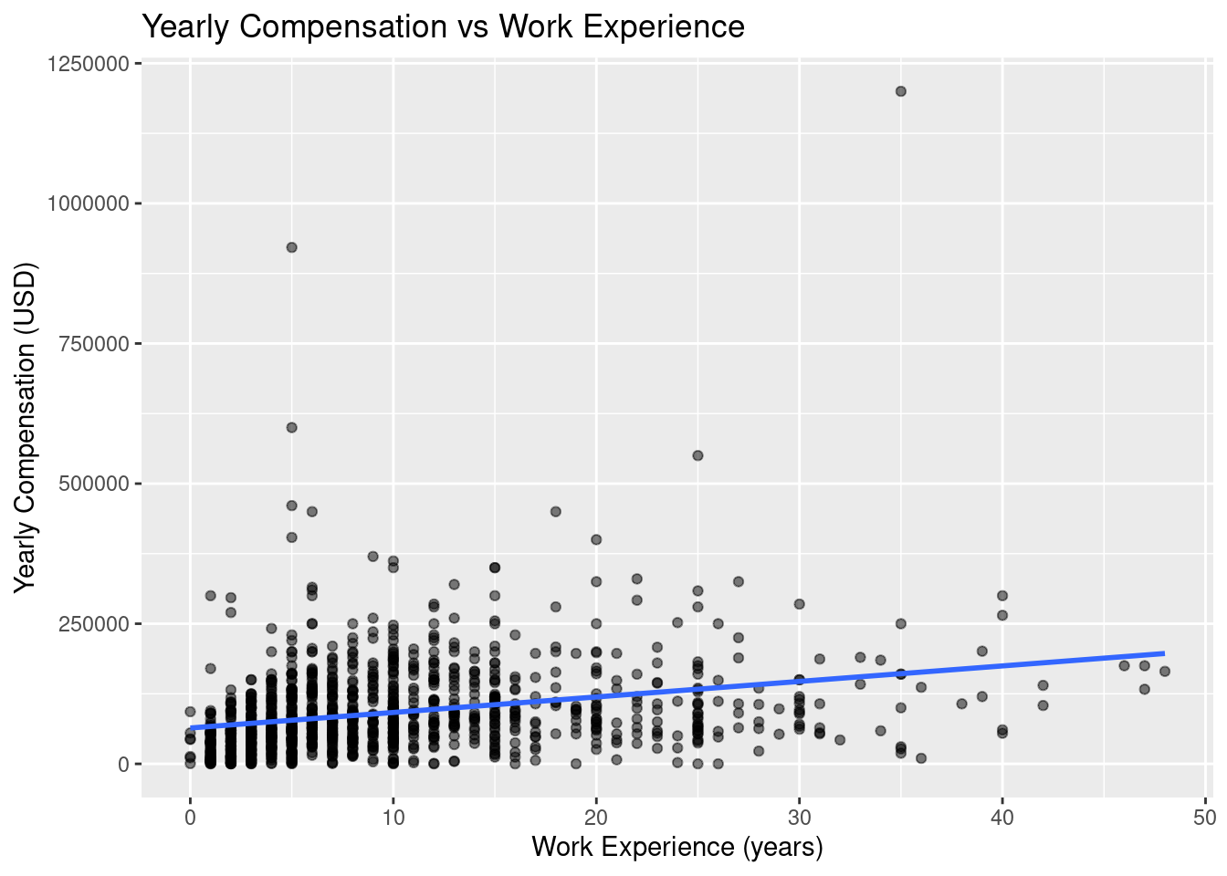
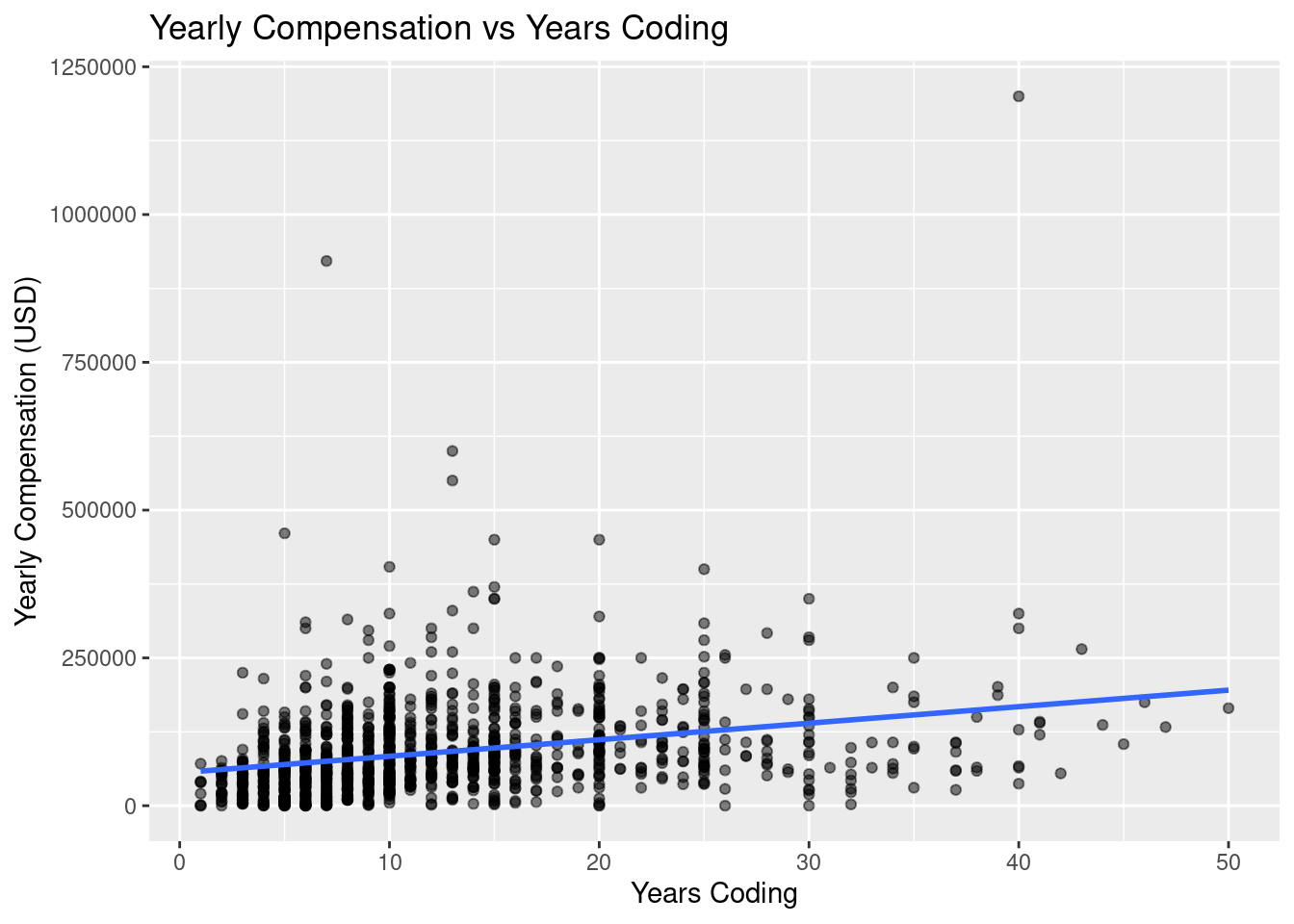
$ converted_comp_yearly <dbl> 3237, 52046, 74963, 56757, 74963, 132260, 117798, 165974, 64254, 71779, 36351, 81349, 10…
$ work_exp              <dbl> 10, 7, 16, 17, 7, 25, 3, 7, 13, 10, 10, 13, 10, 19, 3, 14, 3, 5, 5, 2, 25, 30, 11, 2, 3,…
$ years_code            <dbl> 14, 7, 8, 29, 7, 25, 13, 8, 22, 10, 3, 13, 8, 19, 3, 3, 7, 10, 15, 7, 27, 40, 15, 4, 7, …
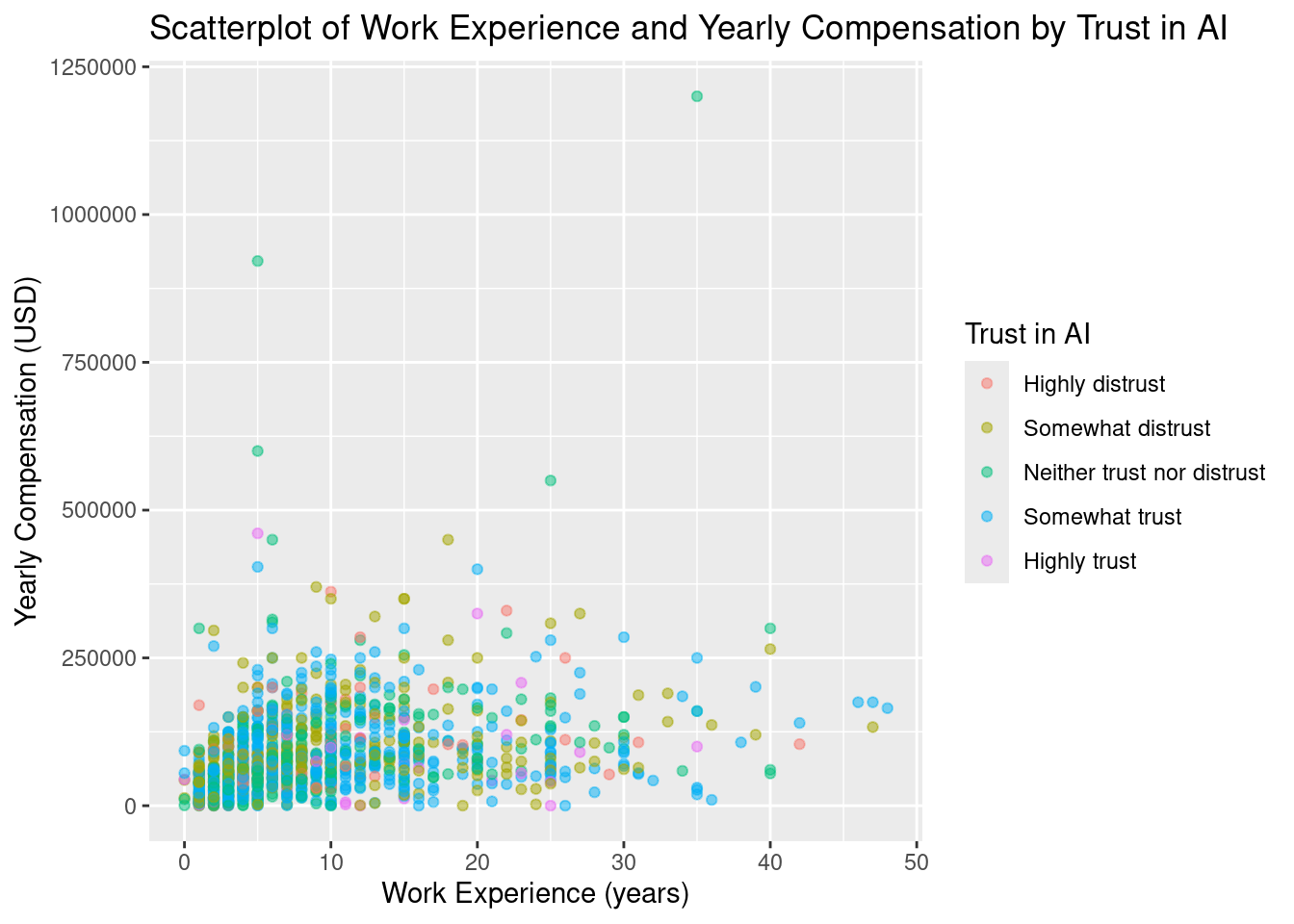
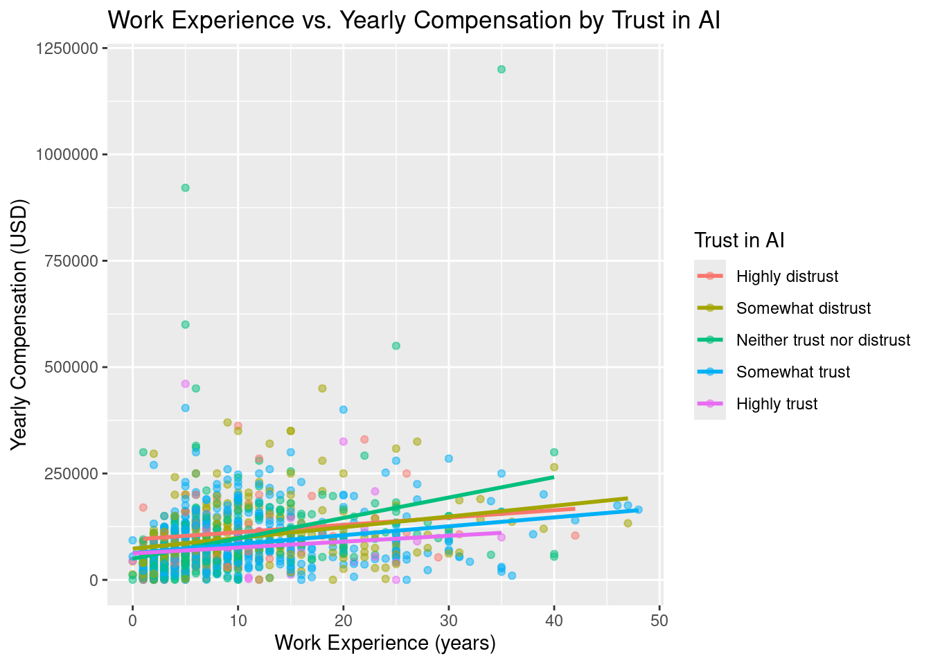
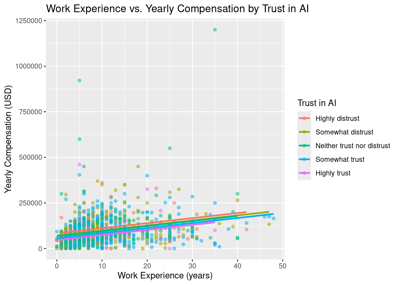
$ ai_trust              <fct> Somewhat trust, Somewhat trust, Somewhat trust, Somewhat trust, Somewhat trust, Neither …

4. Summary Statistics

# Summarize mean and median values for converted_comp_yearly and work_exp
data_dev_survey |>
  summarize(mean_comp = mean(converted_comp_yearly),
            median_comp = median(converted_comp_yearly),
            mean_exp = mean(work_exp),
            median_exp = median(work_exp))
# A tibble: 1 × 4
  mean_comp median_comp mean_exp median_exp
      <dbl>       <dbl>    <dbl>      <dbl>
1    90702.      72768.     9.65          7

5. Using tidy_summary() Function

# Use tidy_summary to get a clean summary of the two columns
data_dev_survey |>
  select(converted_comp_yearly, work_exp) |>
  tidy_summary()
# A tibble: 2 × 11
  column                    n group type      min     Q1     mean median     Q3     max       sd
  <chr>                 <int> <chr> <chr>   <dbl>  <dbl>    <dbl>  <dbl>  <dbl>   <dbl>    <dbl>
1 converted_comp_yearly  1182 <NA>  numeric     3 41390. 90702.   72768. 120000 1200000 81928.  
2 work_exp               1182 <NA>  numeric     0     4      9.65     7      13      48     8.19

6. Correlation Between Salary and Work Experience

# Compute the correlation between converted_comp_yearly and work_exp
data_dev_survey |>
  get_correlation(formula = converted_comp_yearly ~ work_exp)
# A tibble: 1 × 1
    cor
  <dbl>
1 0.277

7. Scatterplot of Salary and Work Experience

# Plot the relationship between work experience and yearly compensation
ggplot(data_dev_survey, aes(x = work_exp, y = converted_comp_yearly)) +
  geom_point(alpha = 0.2) +
  labs(x = "Work Experience (years)", y = "Yearly Compensation (USD)",
       title = "Scatterplot of Work Experience and Yearly Compensation")


8. Regression Line

# The same scatterplot with a regression line added
ggplot(data_dev_survey, aes(x = work_exp, y = converted_comp_yearly)) +
  geom_point(alpha = 0.2) +
  geom_smooth(method = "lm", se = FALSE) +
  labs(x = "Work Experience (years)", y = "Yearly Compensation (USD)",
       title = "Work Experience vs. Yearly Compensation with Regression Line")
`geom_smooth()` using formula = 'y ~ x'


9. Fit a Regression Model

# Fit a linear regression model with compensation as the outcome
salary_slr_model <- lm(converted_comp_yearly ~ work_exp, data = data_dev_survey)

# Get the regression coefficients
coef(salary_slr_model)
(Intercept)    work_exp 
  63973.960    2769.115 

Session 5: Multiple Linear Regression Analysis (Part 1)

10: Fitting a Simple Linear Regression with a Categorical Regressor

# Fit a simple linear regression model with ai_trust as a predictor on salary
trust_model <- lm(converted_comp_yearly ~ ai_trust, data = data_dev_survey)

# Get regression coefficients
coef(trust_model)
                       (Intercept)          ai_trustSomewhat distrust ai_trustNeither trust nor distrust 
                         113080.86                          -14688.72                          -20883.40 
            ai_trustSomewhat trust               ai_trustHighly trust 
                         -29605.58                          -35437.81 

11: Visualizing Data with Categorical Variable

# Scatterplot with ai_trust as color for grouping on work_exp predicting
# converted_comp_yearly
ggplot(data_dev_survey, 
       aes(x = work_exp, y = converted_comp_yearly, color = ai_trust)) +
  geom_point(alpha = 0.5) +
  labs(x = "Work Experience (years)", y = "Yearly Compensation (USD)",
       color = "Trust in AI",
       title = "Scatterplot of Work Experience and Yearly Compensation by Trust in AI")


12: Summarizing the Target and Regressors (One numerical and one categorical)

# Summarize the target and regressors
data_dev_survey |>
  select(converted_comp_yearly, work_exp, ai_trust) |>
  tidy_summary()
# A tibble: 7 × 11
  column                    n group                      type      min     Q1     mean median     Q3     max       sd
  <chr>                 <int> <chr>                      <chr>   <dbl>  <dbl>    <dbl>  <dbl>  <dbl>   <dbl>    <dbl>
1 converted_comp_yearly  1182 <NA>                       numeric     3 41390. 90702.   72768. 120000 1200000 81928.  
2 work_exp               1182 <NA>                       numeric     0     4      9.65     7      13      48     8.19
3 ai_trust                 66 Highly distrust            factor     NA    NA     NA       NA      NA      NA    NA   
4 ai_trust                270 Somewhat distrust          factor     NA    NA     NA       NA      NA      NA    NA   
5 ai_trust                319 Neither trust nor distrust factor     NA    NA     NA       NA      NA      NA    NA   
6 ai_trust                489 Somewhat trust             factor     NA    NA     NA       NA      NA      NA    NA   
7 ai_trust                 38 Highly trust               factor     NA    NA     NA       NA      NA      NA    NA   

13: Fitting a Multiple Regression Model with Interaction Terms

# Fit a multiple regression model with interaction
multi_model_interaction <- lm(converted_comp_yearly ~ work_exp * ai_trust, 
                              data = data_dev_survey)

# Get regression coefficients
coef(multi_model_interaction)
                                (Intercept)                                    work_exp 
                                 94685.6495                                   1724.5513 
                  ai_trustSomewhat distrust          ai_trustNeither trust nor distrust 
                                -21369.0390                                 -44973.0562 
                     ai_trustSomewhat trust                        ai_trustHighly trust 
                                -31608.7285                                 -32523.5905 
         work_exp:ai_trustSomewhat distrust work_exp:ai_trustNeither trust nor distrust 
                                   792.3242                                   3069.4610 
            work_exp:ai_trustSomewhat trust               work_exp:ai_trustHighly trust 
                                   370.1143                                   -343.6176 

14: Adding Interaction Terms to the Regression Plot

# Scatterplot with regression lines by trust in AI
ggplot(data_dev_survey, aes(x = work_exp, y = converted_comp_yearly, color = ai_trust)) +
  geom_point(alpha = 0.5) +
  geom_smooth(method = "lm", se = FALSE) +
  labs(x = "Work Experience (years)", y = "Yearly Compensation (USD)",
       color = "Trust in AI",
       title = "Work Experience vs. Yearly Compensation by Trust in AI")
`geom_smooth()` using formula = 'y ~ x'


Session 6: Multiple Linear Regression Analysis (Part 2)

15. Fitting a Multiple Regression Model Without Interactions

# Fit a multiple regression model without interaction terms
multi_model_no_interaction <- lm(converted_comp_yearly ~ work_exp + ai_trust, 
                                 data = data_dev_survey)

# Get regression coefficients
coef(multi_model_no_interaction)
                       (Intercept)                           work_exp          ai_trustSomewhat distrust 
                         83491.170                           2774.034                         -12736.618 
ai_trustNeither trust nor distrust             ai_trustSomewhat trust               ai_trustHighly trust 
                        -15877.388                         -27030.100                         -36946.496 

16. Visualizing the Parallel Slopes Model

# Scatterplot with regression lines by trust in AI (parallel slopes)
ggplot(data_dev_survey, aes(x = work_exp, y = converted_comp_yearly, color = ai_trust)) +
  geom_point(alpha = 0.5) +
  geom_parallel_slopes(se = FALSE) +
  labs(x = "Work Experience (years)", y = "Yearly Compensation (USD)",
       color = "Trust in AI",
       title = "Work Experience vs. Yearly Compensation by Trust in AI")


17. Summarize the Numerical Regressors and Target Variable

# Use tidy_summary to get a clean summary of the data for a multiple regression
# with work experience and years coding as regressors and yearly compensation as
# the outcome
data_dev_survey |>
  select(converted_comp_yearly, work_exp, years_code) |>
  tidy_summary()
# A tibble: 3 × 11
  column                    n group type      min     Q1     mean median     Q3     max       sd
  <chr>                 <int> <chr> <chr>   <dbl>  <dbl>    <dbl>  <dbl>  <dbl>   <dbl>    <dbl>
1 converted_comp_yearly  1182 <NA>  numeric     3 41390. 90702.   72768. 120000 1200000 81928.  
2 work_exp               1182 <NA>  numeric     0     4      9.65     7      13      48     8.19
3 years_code             1182 <NA>  numeric     1     7     12.5     10      16      50     8.38

18. Fitting a Multiple Regression Model with Two Numerical Predictors

# Fit a multiple regression model
multi_model <- lm(converted_comp_yearly ~ work_exp + years_code, 
                  data = data_dev_survey)

# Get regression coefficients
coef(multi_model)
(Intercept)    work_exp  years_code 
  55764.220    1343.020    1753.121 

19. Visualizing the Relationship between Variables (with SLR)

# Create scatterplots with regression lines for both variables with 
# converted_comp_yearly as the response variable in simple linear regression
ggplot(data_dev_survey, aes(x = work_exp, y = converted_comp_yearly)) +
  geom_point(alpha = 0.5) +
  geom_smooth(method = "lm", se = FALSE) +
  labs(x = "Work Experience (years)", y = "Yearly Compensation (USD)",
       title = "Yearly Compensation vs Work Experience")
`geom_smooth()` using formula = 'y ~ x'

ggplot(data_dev_survey, aes(x = years_code, y = converted_comp_yearly)) +
  geom_point(alpha = 0.5) +
  geom_smooth(method = "lm", se = FALSE) +
  labs(x = "Years Coding", y = "Yearly Compensation (USD)",
       title = "Yearly Compensation vs Years Coding")
`geom_smooth()` using formula = 'y ~ x'